PCS Dispatch Efficiency
How one PCS efficiency curve turns into different realized values depending on dispatch.
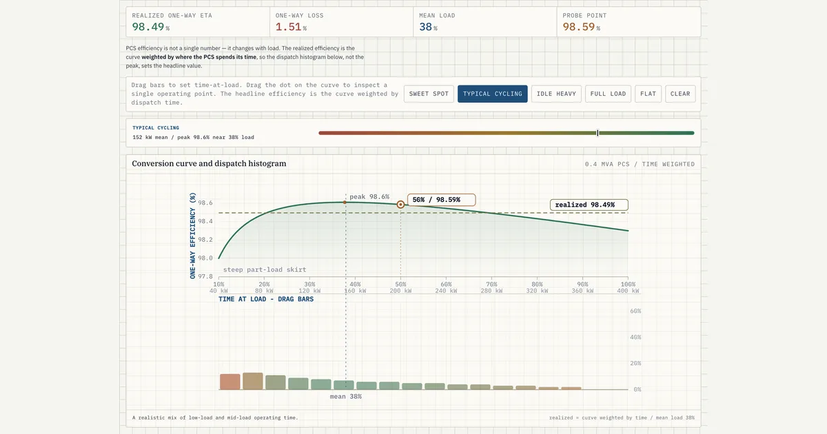
PCS efficiency is not a single number — it changes with load. The realized efficiency is the curve weighted by where the PCS spends its time, so the dispatch histogram below, not the peak, sets the headline value.
Download the PCS Dispatch Efficiency diagram
Free to download and reuse — including commercially — under CC BY 4.0, with credit to BESS.engineer. Licence & attribution →
Browse all BESS diagrams →
What it shows
Realized PCS efficiency is a single 0.4 MVA power-conversion-system efficiency curve, weighted by how much time the PCS actually spends at each load. The curve runs roughly 98.0% to 98.6% one-way, rising off a part-load skirt to a mid-load peak (about 98.6% near 38% load) and easing slightly past it. A dispatch histogram below marks time-at-load, and the realized figure is the time-weighted average of the curve. Pick a profile, drag histogram bars, or move a curve probe.
Why it matters for BESS
Datasheets quote a peak or headline PCS efficiency, but a battery almost never sits at that load. The efficiency it realizes is set by its dispatch pattern: an idle-heavy profile parks most of its hours on the low-load skirt where conversion is worst, while a full-load or sweet-spot profile keeps time near the peak. This one-way conversion loss is separate from the battery's round-trip efficiency and compounds with it on both charge and discharge.
How to read it
The green line is the efficiency curve; the amber histogram is time-at-load. The realized-eta readout is the curve weighted by that histogram, with mean load shown alongside. Move the accent probe to read the curve at any single load point, and compare it to the realized value: they only match if all time sits in one bin. Switching from Sweet spot to Idle heavy drops realized efficiency as weight shifts left onto the part-load skirt.
Frequently asked
- Why is realized PCS efficiency different from the peak on the datasheet?
- Because efficiency changes with load, and a battery rarely holds the load that produces peak efficiency. The realized value is the efficiency curve weighted by how much time the PCS spends at each load, so an idle-heavy dispatch that dwells on the low-load skirt realizes a lower number than the nameplate peak. Only a profile concentrated at the peak load would come close to the headline figure.
- Is this the same as round-trip efficiency?
- No. This is a one-way PCS conversion efficiency — the loss the power-conversion system takes in a single direction, charge or discharge. Round-trip efficiency (RTE) is roughly charge efficiency times discharge efficiency across the whole system, including the battery. The PCS one-way figure shown here is one factor inside RTE, applied on each leg, not the round trip itself.
- How does dispatch profile change the realized efficiency?
- Dispatch decides where the histogram weight sits on the curve. A Full-load or Sweet-spot profile keeps most hours near the mid-to-high load peak, so realized efficiency stays high. An Idle-heavy profile puts most time at very low load on the part-load skirt, where a fixed offset loss is a large fraction of a small output, dragging the weighted average down.
- What does the curve probe tell me?
- The probe reads the efficiency curve at one specific load point, independent of dispatch. It answers 'what is efficiency at this load' rather than 'what does the whole profile realize'. The probe and the realized-eta readout only agree when all the dispatch time sits in a single load bin; any spread of time across loads makes the weighted realized value differ from any single probe point.
References
Standards and authoritative sources this visual is built on:
- EN 50530: Overall efficiency of grid connected photovoltaic inverters
- IEC 61683: Photovoltaic systems — Power conditioners — Procedure for measuring efficiency
- Performance Test Protocol for Evaluating Inverters Used in Grid-Connected Photovoltaic Systems (origin of the CEC weighted-efficiency scheme)
- IEC 62933-2-1: Electrical energy storage (EES) systems — Part 2-1: Unit parameters and testing methods — General specification (round-trip efficiency)